通过Amber, AmberTools以及VMD模拟离子液体径向分布函数(RDFs)
Room-temperature ionic liquids are, as the name suggests, salts that exist in liquid states at room temperature. RTILs are of great interest to a variety of fields because they exhibit unique physical and thermodynamic properties, such as negligble vapor pressure, high thermal stability, high electrochemical stability, and low flammability. Moreover, ionic liquids exhibit high conductivity and a wide electrochemical window, which means that they are neither easily oxidized nor reduced, hence they are excellent candidates for efficient and green electrolytes in batteries. Due to the various potential applications RTILs promise, computer simulations of RTILs have widely propagated, and various combinations of different cations and anions have been designed and tested to further increase our knowledge in this field.
In this tutorial, we will be generating an ionic liquid mixture of 1-Butyl-3-methylimidazolium tetrafluoroborate ([bmim][BF4]) and Acetonitrile (CH3CN) to replicate the data in the paper: X. Wu, Z. Liu, S. Huang and W. Wang, “Molecular dynamics simulation of room-temperature ionic liquid mixture of [bmim][BF4] and acetonitrile by a refined force field”, Phys. Chem. Chem. Phys 7, 2771-2779 (2005). See also Z. Liu, S. Huang and W. Wang, “A refined force field for molecular simulation of imidazolium-based ionic liquids”, J. Phys. Chem. B 108, 12978-12989 (2004).
Please note: this tutorial uses the general Amber force field (GAFF) force field to create an initial (not a “refined”) force field. Some aspects of the simulation results are not in as good agreement with experiment as the results presented in the papers listed above. This is a good object lesson: GAFF can get you started, and can provide results of reasonable accuracy. Depending on your needs, this may be enough. But it is often desirable to treat the GAFF results as a starting point for further refinement; the latter is usually system-specific, and is not covered in this tutorial.
1 Creating initial structures
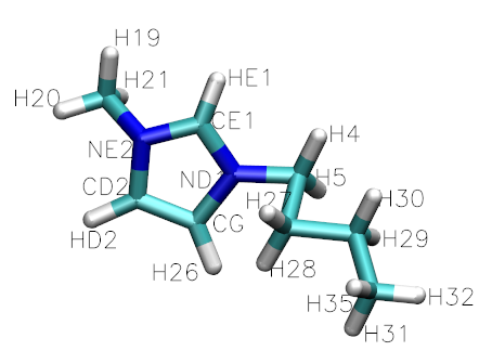
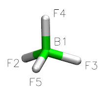

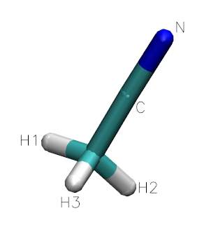
Figure 1:
Structures of the ionic liquid component molecules
1.1 Drawing the molecules using xleap
We will use xleap to draw the molecules and to generate pdb files. First type “xleap” at the command prompt to bring up a window like this one:
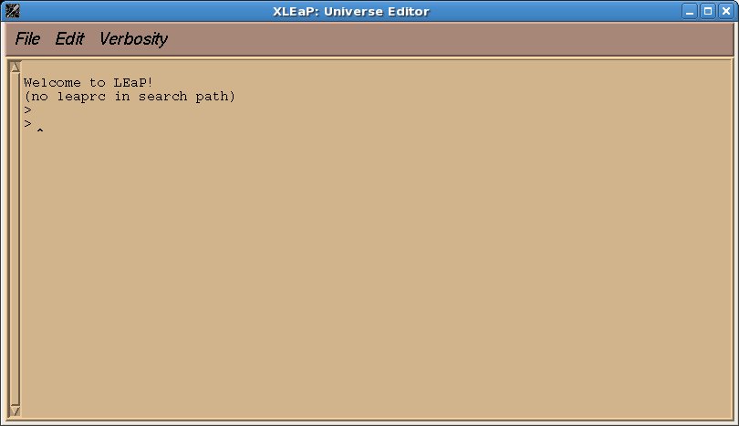
Figure 2:
Next, we will create our first unit, by typing at the xleap command prompt:
edit BF4
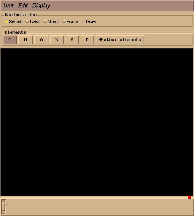
Figure 3:
This will create an “BF4” object, and a graphical interface will open pop up. Drawing a molecule is fairly intuitive: select “draw” in the “Manipulation” box, select an appropriate element, click to draw an atom, and drag to draw a bond. For BF4, select “Boron” from “other elements,” and left click to draw a single boron atom.
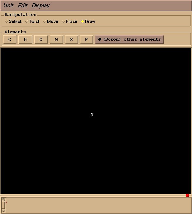
Figure 4:
Next, select “Fluorine” from “other elements,” and drag your mouse from the boron atom to the desired fluorine position.
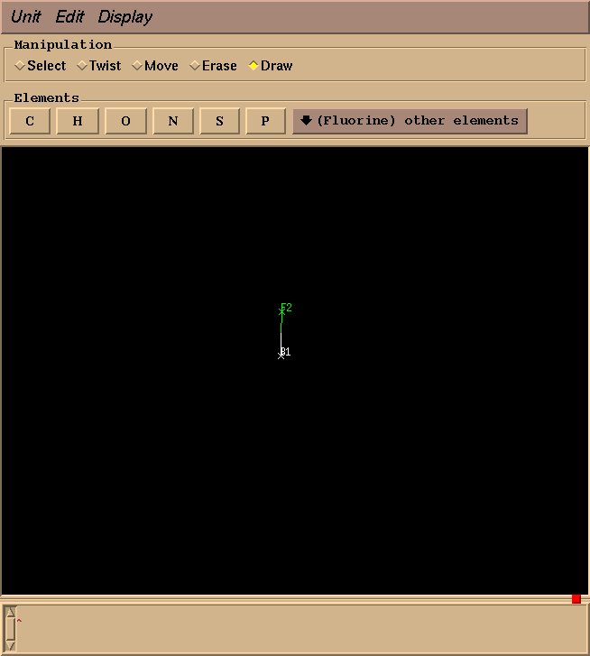
Figure 5:
Draw three more fluorine atoms in the same manner, roughly in a tetrahedral geometry. The geometry need not be perfect at this stage–rough estimations will suffice.
Note: Hold control and move the mouse to rotate the view. Hold control and the right mouse while moving the mouse upwards to zoom in or downwards to zoom out. If you click an atom and select it, hold shift and click anywhere in the drawing space to deselect.
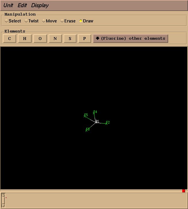
Figure 6:
Xleap will optimise the geometry for us. Select all atoms by dragging your mouse over the molecule (or by clicking each atom). Select “Relax selection” under the “Edit” menu.
Note: The menu may not work properly if the NUM/CAPS Lock is turned on.
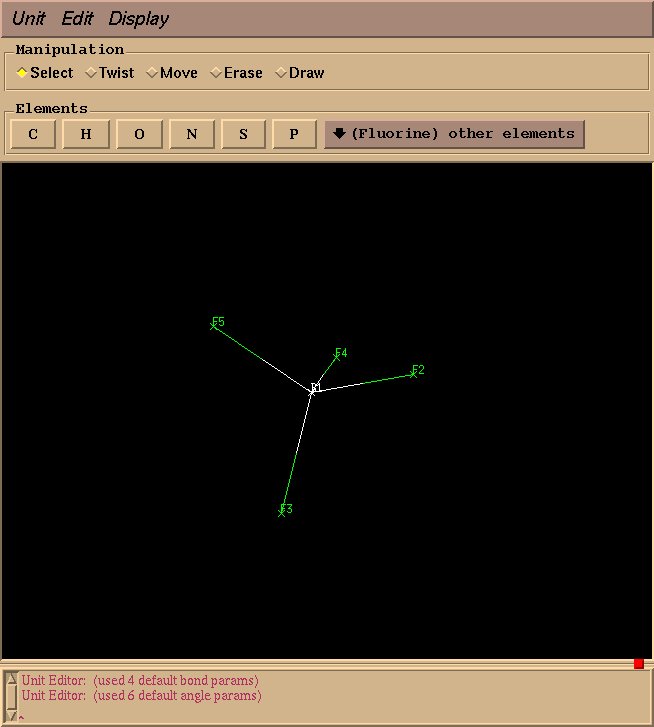
Figure 7:
Exit out of this window. Note: Do NOT use the “X” button, as xleap will quit in entirety and your work will not be saved. Instead, select “Close” under unit.
1.2 Creating a pdb file
To create the pdb file for our molecule, type in the following command:
savePdb BF4 bf4.pdb
1.3 Repeat
Repeat steps 1 and 2 for the two remaining molecules.
(Note: in this tutorial, we use acn for Acetonitrile, bmi for bmim, and bf4 for BF4.)
2 Antechamber
antechamber -help (allows you to learn about antechamber)
2.1 Generate mol2 and frcmod files for the Acetonitrile:
The mol2 contains charge information to be used in LeaP. The following commands will create a mol2 files from the pdb files:
To create the pdb file for our molecule, type in the following command: used in LeaP. The following commands will create a mol2 files from the pdb files:
antechamber –i acn.pdb -fi pdb -o acn.mol2 -fo mol2 -c bcc -nc 0
(-i is input, -fi is input format, -o is output, -fo is output format, -c is charge method, and -nc is net molecular charge. Don’t forget to use “-nc 1” or “-nc -1” for cations and anions, respectively.)
2.2 Problems with boron
Antechamber does not recognize boron, so we’ll need to enter in the parameters ourselves. Our reference paper contains charges for each atom, so we’ll use these numbers.
2.2.1 Run antechamber without the charge model
Type in:
antechamber -i bf4.pdb -fi pdb -o bf4.mol2 -fo mol2
2.2.2 Edit the mol2 file
Using your preferred text editor (e.g., vim or gedit), open bf4.mol2. We’ll need to make few changes:
First, if the second digit in the third line of the file is a “0,” change it to 4. This means that our molecule will have four bonds (four fluorines bonded to boron).
Second, locate the last column in the “Atoms” category. These numbers represent each atom’s charge. As of now, they’re all zeros since we didn’t identify a charge model. Correct the charges by replacing this column with the numbers provided in the paper. (Boron: 1.1504, Fluorine: -0.5376).
Finally, we’ll need to add in the bonds manually. Bonds are specified by the bond id, two atom numbers (the first column in the atom section), and the bond type (1 for single bond, 2 for double bond, etc.)
Add a record under the “Bonds” category:
1 1 2 1
This would be the first record (the first number) that says that the B1 atom (the second number) and the F2 atom (the third number) will form a single bond (the fourth number).
Add three more records:
1 1 3 1
1 1 4 1
1 1 5 1
Note: Bond ids are all 1’s, as the bond ids are of no significance in this case.
2.3 Next, go to xLEaP and put in:
ACN = loadmol2 acn.mol2 #this loads the mol2 file
edit ACN #allows you to visualize the molecule, look for any problems
quit #quit xLEaP
Generate mol2 files for bmim and BF4 by using antechamber and substituting input and output names with appropriate names. Repeat steps 1 and 2 for each molecule. You can get the mol2 files we created here: acn.mol2, bmi.mol2, and bf4.mol2. Compare them to the ones you have created.
3 Parmchk
Parmchk creates force field modification (frcmod) files that fill in missing parameters. The following command creates a frcmod file from the previously created mol2 file:
parmchk -i acn.mol2 -f mol2 -o frcmod.acn
Repeat this step for the two remaining mol2 files. You can get the frcmod files we created here: frcmod.acn, frcmod.bmi, and frcmod.bf4. Compare them to the ones you have created. Note that the frcmod.acn file is essentially empty, since all of the parameters needed for that molecule were present in the gaff.dat file. You can get rid of this file if you want.
4 Packmol
“Packmol creates an initial point for molecular dynamics simulations by packing molecules in defined regions of space. The packing guarantees that short range repulsive interactions do not disrupt the simulations”.
- Download Packmol from http://www.ime.unicamp.br/~martinez/packmol/ and follow the installation instructions.
- Create an input file named input.inp. Here is an example:
tolerance 2.0 # tolerance distance
output ionic2.pdb # output file name
filetype pdb # output file type
#
# Create a box of [bmim][BF4] and acetonitrile molecules
#
structure bf4.pdb
number 102 # Number of molecules
inside cube 0. 0. 0. 35. # x, y, z coordinates of box, and length of box in Angstroms
end structure
# bmim
structure bmi.pdb
number 102
inside cube 0. 0. 0. 35.
end structure
# acetonitrile
structure acn.pdb
number 154
inside cube 0. 0. 0. 35.
end structure
- Run Packmol
$ packmol < input.inp
- View the pdb file generated by packmol in Visual Molecular Dynamics (VMD):
e
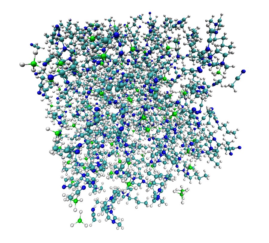
Figure 8:
Structure arising from packmol
5 Using tLEaP to generate Amber prmtop file
With the newly synthesized pdb file from packmol, use tLEaP to generate a parameter-topology file (prmtop) and a coordinates file (inpcrd).
- Create an input file, commands.in:
# change location of files accordingly
source leaprc.gaff
BMI = loadmol2 bmi.mol2
BF4 = loadmol2 bf4.mol2
ACN = loadmol2 acn.mol2
ionicbox = loadPdb ionicbox.pdb
loadamberparams frcmod.bf4
loadamberparams frcmod.bmi
loadamberparams frcmod.acn
setbox ionicbox centers
saveAmberParm ionicbox ionicbox.prmtop ionicbox.inpcrd
- Run tLEaP with input file:
$ tleap -f commands.in
6 Performing minimization with Sander
- Create a script named runmin.sh. This script will create the input file and run sander. “imin=1” tells sander to run minimization, “ntpr=100” saves the restart file every 100 steps, “ntwx=100” prints the trajectory every 100 steps, “maxcyc=10000” runs minimization for 10000 cycles, and “ntb=1” specifies periodic boundary conditions.
- Note: Make sure you modify the arguments for sander if you want to run a second simulation. For example, after “min1” finishes, the input coordinate file should be “min1.x”, and the other output files should begin with “min2”.
#!/bin/bash
# CREATE the mdin file
cat > mdin << EOF
minimization
&cntrl
imin=1, ntpr=100, ntwx=100, maxcyc=10000,
ntb=1,
&end
EOF
sander -O \
-i mdin.in \ # input file
-o min1.o \ # output file
-p ionicbox.prmtop \ # topology file
-c ionicbox.inpcrd \ # input coordinate file
-r min1.x \ # restart file
-x min1.nc \ # output coordinate sets saved in trajectory
-e min1.dat # energy data
Run this with:
$ ./runmin.sh
You should take a look at the Amber manual to learn more about these parameters.
7 Running Molecular Dynamics
- Create script file named runmd.sh
#!/bin/bash
# CREATE the mdin file
cat > mdin << EOF
equilibration for box
&cntrl
imin=0, ntpr=3000, ntwx=3000,
ntx=1, irest=0,
tempi=298., temp0=298., ntt=3,
gamma_ln=5., ntb=2, ntp=1, taup=1.0, ioutfm=1, nstlim=3000000,
ntwr=1000, dt=.001, ig=-1,
/
EOF
# Run sander command.
sander -O \
-i mdin \
-o md1.out \
-p ionicbox.prmtop \
-c min1.x \ # The restart file from minimization
-r md1.x \$RUN.rst7
-x md1.nc \
-e md1.dat
Once again, you should look at the Amber manual to understand what exactly this input file is doing.
Note: The restart file generated from MD simluations contains velocity information that the restart file from minimization did not have. To address this difference, use ntx=5 and irest=1 for future simulations to denote that the restart file (that is, the new input coordinates file) indeed contains the velocity information for sander to process.
Also note: when you run the next simulation, use the restart file from the previous output as your new input coordinates file.
8 Imaging with ptraj
The box we created with packmol manifests a fundamental problem: a significant portion of the molecules is exposed to vacuum, which would yield deviations in simulation results. Under periodic boundaries, our box is “replicated” in all three dimensions so that our system represents a realistic bulk fluid. As a result, when a molecule exits the box from one side, it enters from the other. Ptraj’s imaging tool repacks the molecules that left the box and gives us a proper image of what the central box looks like.
Create an input file, “ptraj.in”:
trajin md1.nc # the name of the trajectory
image center
trajout ptraj.out # the name of the output filethe
To run ptraj, run the following command:
ptraj prmtop ptraj.in
Ptmtop is the topology file for our box.
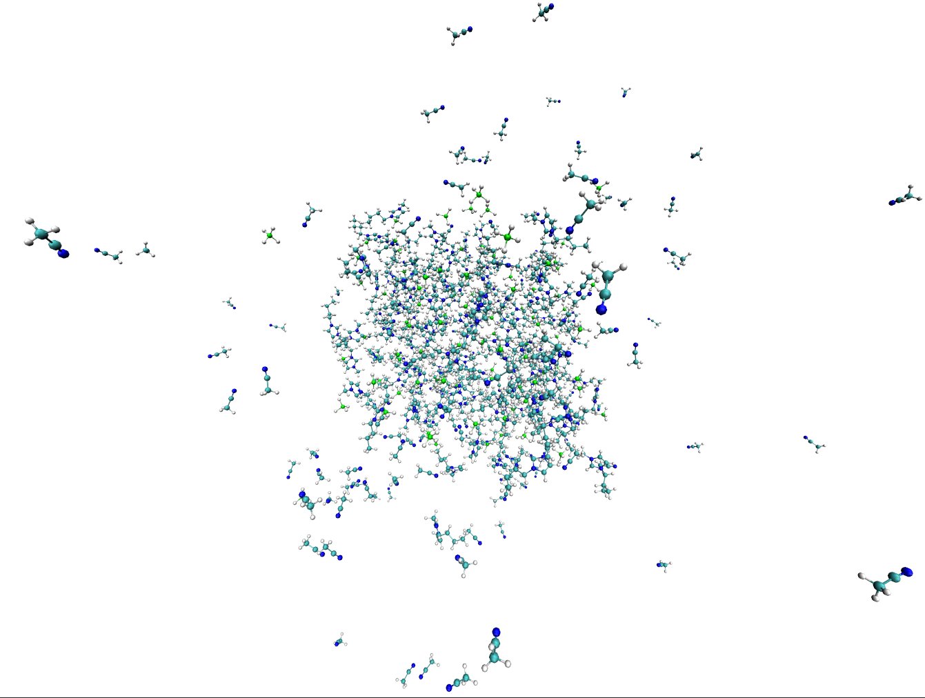
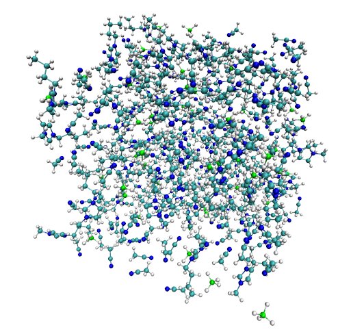
Figure 9:
MD results: (left) before imaging in ptraj; (right) after imaging
Radial Distribution Functions (RDFs)
- First, analyze the Density to see if the average density is close to your target.
awk ‘/Density/ { print $3 }; $1==”A” && $2==”V” {exit 0}’ md1.out > density.dat
This awk script takes in the input file (md1.out) and prints the third column everytime the word “Density” appears in a line. The output is channeled into “density.dat”. When awk reaches the “Average” section in the output file, the script quits.
- To graph density data with xmgrace:
$ xmgrace density.dat
- To calculate the average density, examine the sets in xmgrace, or run the following script:
awk ‘{ sum = sum + $1 }; END { print “average = “, sum/NR }’ density.dat
This awk script takes in density.dat, and adds the first column of each line to “sum”, then prints sum divided by NR (a special variable for Number of Records).
- Examine the Energy Total to see if the system is at equilibrium.
awk ‘/Etot/ {print $3}; ($1==”A” && $2==”V”) {exit 0};’ Eq2.1.out > etot.dat
To graph the Energy Total data in xmgrace, use commands similar to those above for the density.
Below is an example of the graph of the Energy Totals for the the MD simulation for the ionic liquid mixture of [bmim][BF4] and acetonitrile:
- Once the density is at target and total energy is at equilibrium, calculate Radial Distribution Functions.
- In this case, the average density is 1.0774 cc/mol, whereas the paper’s density is 1.087 cc/mol.
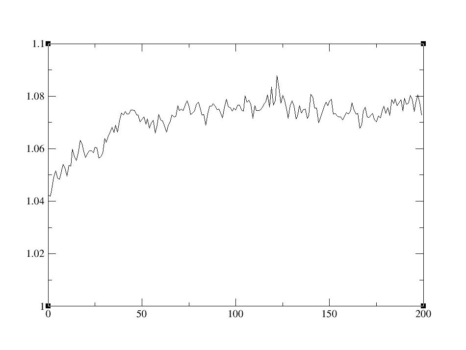
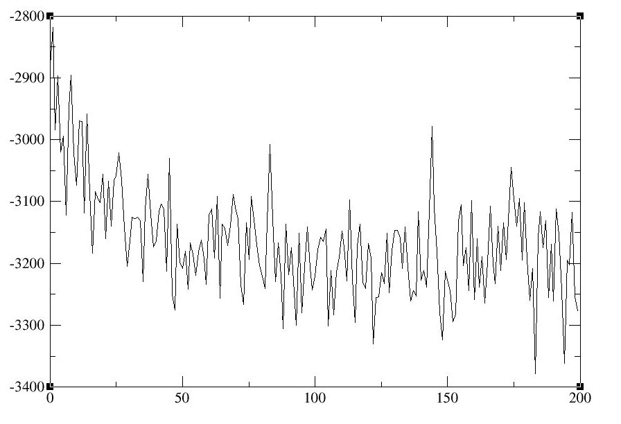
Figure 10:
Time dependence of the density (left) and total energy (right)
In order to calculate the RDFs, we will use ptraj, a program used to analyze sets of 3-D coordinates from input coordinate files. We will be calculating the RDF between the N1 atoms of the Acetonitrile [CH3CN]
- 1) Create an input file ptraj.in
trajin <trajectory filename>
radial CH3CN_N1 .1 15.0 :ACN@N
- 2)Run
ptraj prmtop ptraj.in
CH3CN_N1 is the header for output file names, .1 is the bin size, 15.0 is the maximum for the histogram, and :ACN@N is the mask for selecting atoms we want to use for our analysis.
The output files that result after running the ptraj.in file will be: CH3CN_N1_carnal.xmgr CH3CN_N1_standard.xmgr CH3CN_N1_volume.xmgr
Use Xmgrace to open the files to view the resulting graph of the RDFs. For example:
$ xmgrace CH3CN_N1_volume.xmgr
The above command will open the file CH3CN_N1_volume.xmgr in xmgrace. The x axis is distance in angstroms, and g(r) gives the probablity of finding an atom (in this case, the nitrogen in acetonitrile) at a given distance (r) of another atom (another nitrogen in acetonitrile). The first peak (around four angstroms) represents the first coordination shell, and the second peak (little less than six angstroms) represents the second coordination shell.
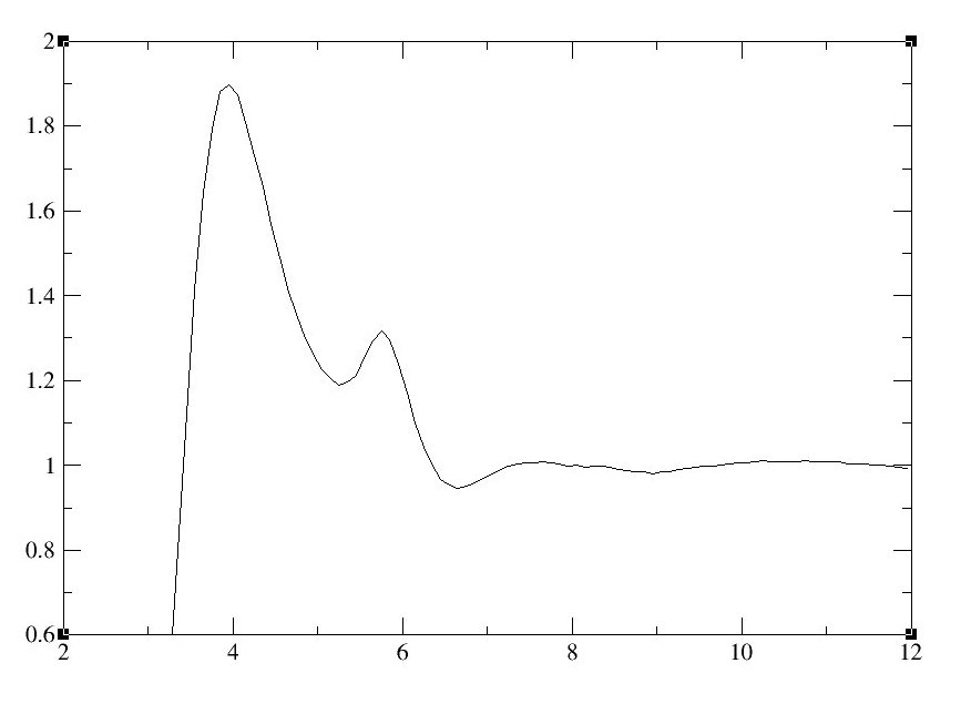
Figure 11:
Radial distribution function
9 Self-Diffusion Coefficients
According to the Einstein relation, the self-diffusion coefficient D can be computed by using the equation below:
D = 1 6 lim t → ∞ d dt <MSD>
in which <MSD> is the averaged mean square displacement.
In order to calculate D, we will 1) Graph the averaged MSD over time using ptraj and gnuplot, 2) Find the slope of the graph, and finally 3) Plug the information into the equation to get D.
9.1 Create the input file
Ptraj will calculate the MSD and print out the x (time) and y (MSD) into a gnuplot-compatible file.
Create a file ptraj.in and type in the following:
trajin trajName # put in the name of your trajectory here (e.g., Eq1.nc)
diffusion mask timestep average
mask is the selection of molecules for analysis. For instance, if you want to calculate D for acetonitrile, replace “mask” with “:ACN”. To calculate D for all residues (which is what this tutorial does), use “:*”.
timestep is dt * ntwx, which gives you the time intervals inbetween entrees in the trajectory (in picoseconds).
9.2 Run ptraj
Run the following command:
ptraj nameOfYourTopologyFile ptraj.in
9.3 Run gnuplot
Open gnuplot (type in gnuplot in the shell). You should see “>” on the left, which means we’re ready to run gnuplot commands.
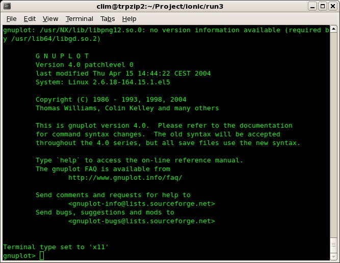
Figure 12:
Type in:
plot ‘diffusion_r.xmgr’ with lines
9.4 Calculate
Using the graph as a reference, calculate the slope of the graph and plug the information into the equation. The units of the slope are angstroms squared over picoseconds.
Note: though the equation suggests that the slope near the end of the graph should be taken, ptraj’s diffusion tool is most accurate at the beginning of the graph. This is somewhat apparent, as noise seems to increase as x increases.
Also note: The thermostat and barostat may disrupt the diffusion coefficient. To get more accurate measurements, run another simulation with the thermostat and barostat turned off.
In this case, the slope is 0.0635990 angstroms squared over picoseconds, or 63.5990 * 10 -11 m 2 over seconds (the units our reference paper uses). To find the diffusion coefficient, we need to divide this number by six, which gives us 10.5998 * 10 -11 m 2 over seconds. In comparison, the reference paper’s diffusion constant is 14.9 * 10 -11 m 2 over seconds. A possible explanation for the difference is that our molecules use general Amber force fields, whereas the paper uses refined force fields.
10 Conclusion
We simulated a room temperature ionic liquid starting from scratch by “hand-drawing” the molecules with xleap, optimizing the geometry with antechamber, generating the topology and coordinates file with xleap/tleap, and running minimization and MD simulations with sander. We also used ptraj to perform analyses on the data we collected, such as calculating RDFs and self-diffusion coefficients, and we used xmgrace and gnuplot to aid us in visualizing the data. Hopefully, by the end of this tutorial, you’ll feel more comfortable with the numerous tools the AMBER suite provides, and you can now move on to more complex simulations (and more complex analyses!).
打赏作者
 微信
微信
 支付宝
支付宝